Navigation Algorithms¶

Kompass, the EMOS navigation engine, provides a comprehensive suite of algorithms for both global path planning and local motion control.

Planning Algorithms – Over 25 sampling-based planners from OMPL (RRT*, PRM, KPIECE, etc.) for global path planning with collision checking.
Control Algorithms – Battle-tested controllers ranging from classic geometric path-followers to GPU-accelerated local planners and visual servoing.

Every algorithm is natively compatible with the three primary motion models. The internal logic automatically adapts to the specific constraints of your platform:

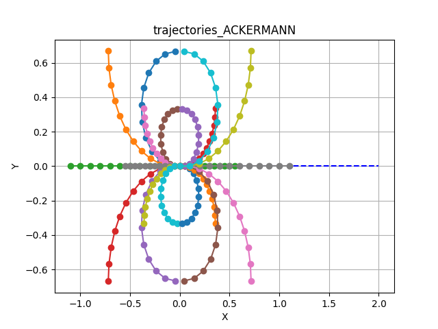
ACKERMANN: Car-like platforms with steering constraints.
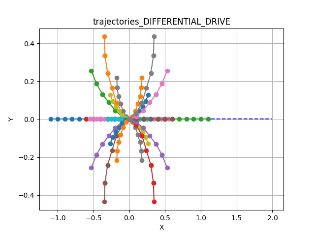
DIFFERENTIAL_DRIVE: Two-wheeled or skid-steer robots.
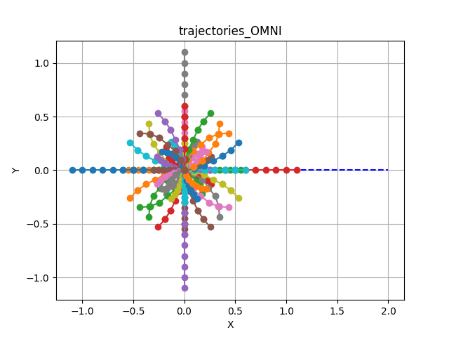
OMNI: Holonomic systems capable of lateral movement.

Each algorithm is fully parameterized. Developers can tune behaviors such as lookahead gains, safety margins, and obstacle sensitivity directly through the Python API or YAML configuration.

Control Algorithms¶

Algorithm	Type	Key Feature	Sensors Required
DWA	Sampling-based planner	GPU-accelerated velocity space planning	LaserScan, PointCloud, OccupancyGrid
Pure Pursuit	Geometric tracker	Lookahead-based path tracking with collision avoidance	LaserScan, PointCloud, OccupancyGrid (optional)
Stanley Steering	Geometric tracker	Front-axle feedback for Ackermann platforms	None (pure path follower)
DVZ	Reactive controller	Deformable safety bubble for fast avoidance	LaserScan
Vision Follower (RGB)	Visual servoing	2D target centering with monocular camera	Detections / Trackings
Vision Follower (RGB-D)	Visual servoing + planner	Depth-aware following with obstacle avoidance	Detections, Depth Image, LaserScan/PointCloud
Trajectory Cost Evaluation	Cost functions	Weighted scoring for sampling-based controllers	–

Dynamic Window Approach (DWA)¶

GPU-accelerated Dynamic Window Approach.

DWA is a classic local planning method developed in the 90s.[1] It is a sampling-based controller that generates a set of constant-velocity trajectories within a “Dynamic Window” of reachable velocities.

EMOS supercharges this algorithm using SYCL-based hardware acceleration, allowing it to sample and evaluate thousands of candidate trajectories in parallel on Nvidia, AMD, or Intel GPUs. This enables high-frequency control loops even in complex, dynamic environments with dense obstacle fields.

It is highly effective for differential drive and omnidirectional robots.

How It Works¶

The algorithm operates in a three-step pipeline at every control cycle:

Compute Dynamic Window. Calculate the range of reachable linear and angular velocities (\(v, \omega\)) for the next time step, limited by the robot’s maximum acceleration and current speed.
Sample Trajectories. Generate a set of candidate trajectories by sampling velocity pairs within the dynamic window and simulating the robot’s motion forward in time.
Score and Select. Discard trajectories that collide with obstacles (using FCL). Score the remaining valid paths based on distance to goal, path alignment, and smoothness.

Supported Sensory Inputs¶

DWA requires spatial data to perform collision checking during the rollout phase.

LaserScan
PointCloud
OccupancyGrid

Parameters and Default Values¶

Name	Type	Default	Description
control_time_step	`float`	`0.1`	Time interval between control actions (sec). Must be between `1e-4` and `1e6`.
prediction_horizon	`float`	`1.0`	Duration over which predictions are made (sec). Must be between `1e-4` and `1e6`.
control_horizon	`float`	`0.2`	Duration over which control actions are planned (sec). Must be between `1e-4` and `1e6`.
max_linear_samples	`int`	`20`	Maximum number of linear control samples. Must be between `1` and `1e3`.
max_angular_samples	`int`	`20`	Maximum number of angular control samples. Must be between `1` and `1e3`.
sensor_position_to_robot	`List[float]`	`[0.0, 0.0, 0.0]`	Position of the sensor relative to the robot in 3D space (x, y, z) coordinates.
sensor_rotation_to_robot	`List[float]`	`[0.0, 0.0, 0.0, 1.0]`	Orientation of the sensor relative to the robot as a quaternion (x, y, z, w).
octree_resolution	`float`	`0.1`	Resolution of the Octree used for collision checking. Must be between `1e-9` and `1e3`.
costs_weights	`TrajectoryCostsWeights`	see defaults	Weights for trajectory cost evaluation.
max_num_threads	`int`	`1`	Maximum number of threads used when running the controller. Must be between `1` and `1e2`.

Note

All previous parameters can be configured when using the DWA algorithm directly in your Python recipe or using a config file (as shown in the usage example).

Usage Example¶

DWA can be activated by setting the algorithm property in the Controller configuration.

dwa.py¶

from kompass.components import Controller, ControllerConfig
from kompass.robot import (
    AngularCtrlLimits,
    LinearCtrlLimits,
    RobotCtrlLimits,
    RobotGeometry,
    RobotType,
    RobotConfig
)
from kompass.control import ControllersID

# Setup your robot configuration
my_robot = RobotConfig(
    model_type=RobotType.ACKERMANN,
    geometry_type=RobotGeometry.Type.BOX,
    geometry_params=np.array([0.3, 0.3, 0.3]),
    ctrl_vx_limits=LinearCtrlLimits(max_vel=0.2, max_acc=1.5, max_decel=2.5),
    ctrl_omega_limits=AngularCtrlLimits(
        max_vel=0.4, max_acc=2.0, max_decel=2.0, max_steer=np.pi / 3)
)

# Set DWA algorithm using the config class
controller_config = ControllerConfig(algorithm="DWA")

# Set YAML config file
config_file = "my_config.yaml"

controller = Controller(component_name="my_controller",
                        config=controller_config,
                        config_file=config_file)

# algorithm can also be set using a property
controller.algorithm = ControllersID.DWA      # or "DWA"

my_config.yaml¶

my_controller:
  # Component config parameters
  loop_rate: 10.0
  control_time_step: 0.1
  prediction_horizon: 4.0
  ctrl_publish_type: 'Array'

  # Algorithm parameters under the algorithm name
  DWA:
    control_horizon: 0.6
    octree_resolution: 0.1
    max_linear_samples: 20
    max_angular_samples: 20
    max_num_threads: 3
    costs_weights:
      goal_distance_weight: 1.0
      reference_path_distance_weight: 1.5
      obstacles_distance_weight: 2.0
      smoothness_weight: 1.0
      jerk_weight: 0.0

Trajectory Samples Generation¶

Trajectory samples are generated using a constant velocity generator for each velocity value within the reachable range to generate the configured maximum number of samples (see max_linear_samples and max_angular_samples in the config parameters).

The shape of the sampled trajectories depends heavily on the robot’s kinematic model:

Ackermann

Car-Like Motion

Note the limited curvature constraints typical of car-like steering.

Differential

Tank/Diff Drive

Includes rotation-in-place (if configured) and smooth arcs.

Omni

Holonomic Motion

Includes lateral (sideways) movement samples.

Rotate-Then-Move

To ensure natural movement for Differential and Omni robots, EMOS implements a Rotate-Then-Move policy. Simultaneous rotation and high-speed linear translation is restricted to prevent erratic behavior.

Best Trajectory Selection¶

A collision-free admissibility criteria is implemented within the trajectory samples generator using FCL to check the collision between the simulated robot state and the reference sensor input.

Once admissible trajectories are sampled, the Best Trajectory is selected by minimizing a weighted cost function. You can tune these weights (costs_weights) to change the robot’s behavior (e.g., sticking closer to the path vs. prioritizing obstacle clearance). See Trajectory Cost Evaluation for details.

Pure Pursuit¶

Geometric path tracking with reactive collision avoidance.

Pure Pursuit is a fundamental path-tracking algorithm. It calculates the curvature required to move the robot from its current position to a specific “lookahead” point on the path, simulating how a human driver looks forward to steer a vehicle.

EMOS enhances the standard implementation (based on Purdue SIGBOTS) by adding an integrated Simple Search Collision Avoidance layer. This allows the robot to deviate locally from the path to avoid unexpected obstacles without needing a full replan.

How It Works¶

The controller executes a four-step cycle:

Find Target – Locate Lookahead. Find the point on the path that is distance \(L\) away from the robot. \(L\) scales with speed (\(L = k \cdot v\)).
Steering – Compute Curvature. Calculate the arc required to reach that target point based on the robot’s kinematic constraints.
Safety – Collision Check. Project the robot’s motion forward using the prediction_horizon to check for immediate collisions.
Avoidance – Local Search. If the nominal arc is blocked, the controller searches through max_search_candidates to find a safe velocity offset that clears the obstacle while maintaining progress.

Supported Sensory Inputs¶

To enable the collision avoidance layer, spatial data is required.

LaserScan
PointCloud
OccupancyGrid

(Note: The controller can run in “blind” tracking mode without these inputs, but collision avoidance will be disabled.)

Configuration Parameters¶

Name	Type	Default	Description
lookahead_gain_forward	`float`	`0.8`	Factor to scale lookahead distance by current velocity (\(L = k \cdot v\)).
prediction_horizon	`int`	`10`	Number of future steps used to check for potential collisions along the path.
path_search_step	`float`	`0.2`	Offset step used to search for alternative velocity commands when the nominal path is blocked.
max_search_candidates	`int`	`10`	Maximum number of search iterations to find a collision-free command.

Usage Example¶

pure_pursuit.py¶

from kompass.components import Controller, ControllerConfig
from kompass.robot import (
    AngularCtrlLimits,
    LinearCtrlLimits,
    RobotCtrlLimits,
    RobotGeometry,
    RobotType,
    RobotConfig
)
from kompass.control import ControllersID, PurePursuitConfig

# Setup your robot configuration
my_robot = RobotConfig(
    model_type=RobotType.OMNI,
    geometry_type=RobotGeometry.Type.BOX,
    geometry_params=np.array([0.3, 0.3, 0.3]),
    ctrl_vx_limits=LinearCtrlLimits(max_vel=0.2, max_acc=1.5, max_decel=2.5),
    ctrl_omega_limits=AngularCtrlLimits(
        max_vel=0.4, max_acc=2.0, max_decel=2.0, max_steer=np.pi / 3)
)

# Initialize the controller
controller = Controller(component_name="my_controller")

# Set the algorithm configuration
pure_pursuit_config = PurePursuitConfig(
        lookahead_gain_forward=0.5, prediction_horizon=8, max_search_candidates=20
    )

controller.algorithms_config = pure_pursuit_config

# NOTE: You can configure more than one algorithm to switch during runtime
# other_algorithm_config = ....
# controller.algorithms_config = [pure_pursuit_config, other_algorithm_config]

# Set the algorithm to Pure Pursuit
controller.algorithm = ControllersID.PURE_PURSUIT

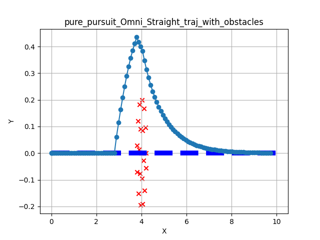
Performance and Results¶

The following tests demonstrate the controller’s ability to track reference paths (thin dark blue) and avoid obstacles (red x).

Nominal Tracking – Performance on standard geometric paths (U-Turns and Circles) without interference:

Ackermann

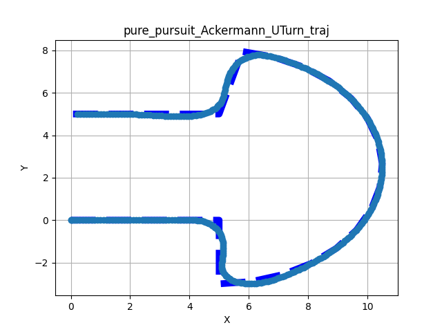
U-Turn

Differential

Circle

Omni

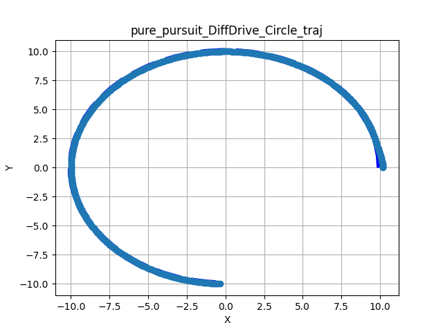
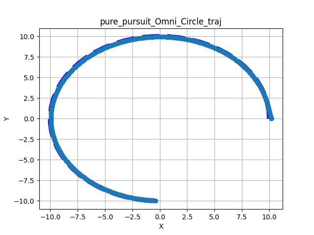
Circle

Collision Avoidance – Scenarios where static obstacles are placed directly on the global path. The controller successfully identifies the blockage and finds a safe path around it:

Ackermann

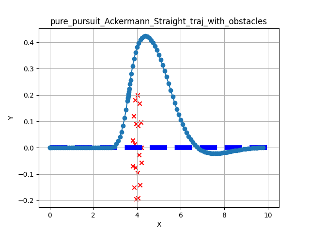
Straight + Obstacles

Differential

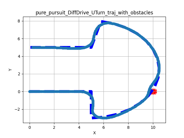
U-Turn + Obstacles

Omni

Straight + Obstacles

Observations

Convergence: Smooth convergence to the reference path across all kinematic models.
Clearance: The simple search algorithm successfully clears obstacle boundaries before returning to the path.
Stability: No significant oscillation observed during avoidance maneuvers.

Stanley Steering¶

Front-wheel feedback control for path tracking.

Stanley is a geometric path tracking method originally developed for the DARPA Grand Challenge.[2] Unlike Pure Pursuit (which looks ahead), Stanley uses the Front Axle as its reference point to calculate steering commands.

It computes a steering angle \(\delta(t)\) based on two error terms:

Heading Error (\(\psi_e\)): Difference between the robot’s heading and the path direction.
Cross-Track Error (\(e\)): Lateral distance from the front axle to the nearest path segment.

The control law combines these to minimize error exponentially:

\[ \delta(t) = \psi_e(t) + \arctan \left( \frac{k \cdot e(t)}{v(t)} \right) \]

Key Features¶

Ackermann Native – Designed specifically for car-like steering geometry. Naturally stable at high speeds for these vehicles.
Multi-Model Support – EMOS extends Stanley to Differential and Omni robots by applying a Rotate-Then-Move strategy when orientation errors are large.
Sensor-Less – Does not require LiDAR or depth data. It is a pure path follower.

Configuration Parameters¶

Name	Type	Default	Description
heading_gain	`float`	`0.7`	Heading gain in the control law. Must be between `0.0` and `1e2`.
cross_track_min_linear_vel	`float`	`0.05`	Minimum linear velocity for cross-track control (m/s). Must be between `1e-4` and `1e2`.
min_angular_vel	`float`	`0.01`	Minimum allowable angular velocity (rad/s). Must be between `0.0` and `1e9`.
cross_track_gain	`float`	`1.5`	Gain for cross-track in the control law. Must be between `0.0` and `1e2`.
max_angle_error	`float`	`np.pi / 16`	Maximum allowable angular error (rad). Must be between `1e-9` and `pi`.
max_distance_error	`float`	`0.1`	Maximum allowable distance error (m). Must be between `1e-9` and `1e9`.

Usage Example¶

stanley.py¶

from kompass.components import Controller, ControllerConfig
from kompass.robot import (
    AngularCtrlLimits,
    LinearCtrlLimits,
    RobotCtrlLimits,
    RobotGeometry,
    RobotType,
    RobotConfig
)
from kompass.control import ControllersID

# Setup your robot configuration
my_robot = RobotConfig(
    model_type=RobotType.ACKERMANN,
    geometry_type=RobotGeometry.Type.BOX,
    geometry_params=np.array([0.3, 0.3, 0.3]),
    ctrl_vx_limits=LinearCtrlLimits(max_vel=0.2, max_acc=1.5, max_decel=2.5),
    ctrl_omega_limits=AngularCtrlLimits(
        max_vel=0.4, max_acc=2.0, max_decel=2.0, max_steer=np.pi / 3)
)

# Set Stanley algorithm using the config class
controller_config = ControllerConfig(algorithm="Stanley")  # or ControllersID.STANLEY

# Set YAML config file
config_file = "my_config.yaml"

controller = Controller(component_name="my_controller",
                        config=controller_config,
                        config_file=config_file)

# algorithm can also be set using a property
controller.algorithm = ControllersID.STANLEY      # or "Stanley"

my_config.yaml¶

my_controller:
  # Component config parameters
  loop_rate: 10.0
  control_time_step: 0.1
  ctrl_publish_type: 'Sequence'

  # Algorithm parameters under the algorithm name
  Stanley:
    cross_track_gain: 1.0
    heading_gain: 2.0

Safety Note

Stanley does not have built-in obstacle avoidance. It is strongly recommended to use this controller in conjunction with the Drive Manager component to provide Emergency Stop and Slowdown safety layers.

Deformable Virtual Zone (DVZ)¶

Fast, reactive collision avoidance for dynamic environments.

The DVZ (Deformable Virtual Zone) is a reactive control method introduced by R. Zapata in 1994.[3] It models the robot’s safety perimeter as a “virtual bubble” (zone) that deforms when obstacles intrude.

Unlike sampling methods (like DWA) that simulate future trajectories, DVZ calculates a reaction vector based directly on how the bubble is being “squished” by the environment. This makes it extremely computationally efficient and ideal for crowded, fast-changing environments where rapid reactivity is more important than global optimality.

How It Works¶

The algorithm continuously computes a deformation vector to steer the robot away from intrusion.

Define Zone – Create Bubble. Define a circular (or elliptical) protection zone around the robot with a nominal undeformed radius \(R\).
Sense – Measure Intrusion. Using LaserScan data, compute the deformed radius \(d_h(\alpha)\) for every angle \(\alpha \in [0, 2\pi]\) around the robot.
Compute Deformation – Calculate Metrics.
- Intrusion Intensity (\(I_D\)): How much total “stuff” is inside the zone. \(I_D = \frac{1}{2\pi} \int_{0}^{2\pi}\frac{R - d_h(\alpha)}{R} d\alpha\)
- Deformation Angle (\(\Theta_D\)): The primary direction of the intrusion. \(\Theta_D = \frac{\int_{0}^{2\pi} (R - d_h(\alpha))\alpha d\alpha}{I_D}\)
React – Control Law. The final control command minimizes \(I_D\) (pushing away from the deformation) while trying to maintain the robot’s original heading towards the goal.

Supported Sensory Inputs¶

DVZ relies on dense 2D range data to compute the deformation integral.

LaserScan

Configuration Parameters¶

DVZ balances two competing forces: Path Following (Geometric) vs. Obstacle Repulsion (Reactive).

Name	Type	Default	Description
min_front_margin	`float`	`1.0`	Minimum front margin distance. Must be between `0.0` and `1e2`.
K_linear	`float`	`1.0`	Proportional gain for linear control. Must be between `0.1` and `10.0`.
K_angular	`float`	`1.0`	Proportional gain for angular control. Must be between `0.1` and `10.0`.
K_I	`float`	`5.0`	Proportional deformation gain. Must be between `0.1` and `10.0`.
side_margin_width_ratio	`float`	`1.0`	Width ratio between the deformation zone front and side (circle if 1.0). Must be between `1e-2` and `1e2`.
heading_gain	`float`	`0.7`	Heading gain of the internal pure follower control law. Must be between `0.0` and `1e2`.
cross_track_gain	`float`	`1.5`	Gain for cross-track error of the internal pure follower control law. Must be between `0.0` and `1e2`.

Usage Example¶

dvz.py¶

from kompass.components import Controller, ControllerConfig
from kompass.robot import (
    AngularCtrlLimits,
    LinearCtrlLimits,
    RobotCtrlLimits,
    RobotGeometry,
    RobotType,
    RobotConfig
)
from kompass.control import LocalPlannersID

# Setup your robot configuration
my_robot = RobotConfig(
    model_type=RobotType.ACKERMANN,
    geometry_type=RobotGeometry.Type.BOX,
    geometry_params=np.array([0.3, 0.3, 0.3]),
    ctrl_vx_limits=LinearCtrlLimits(max_vel=0.2, max_acc=1.5, max_decel=2.5),
    ctrl_omega_limits=AngularCtrlLimits(
        max_vel=0.4, max_acc=2.0, max_decel=2.0, max_steer=np.pi / 3)
)

# Set DVZ algorithm using the config class
controller_config = ControllerConfig(algorithm="DVZ")  # or LocalPlannersID.DVZ

# Set YAML config file
config_file = "my_config.yaml"

controller = Controller(component_name="my_controller",
                        config=controller_config,
                        config_file=config_file)

# algorithm can also be set using a property
controller.algorithm = ControllersID.DVZ      # or "DVZ"

my_config.yaml¶

my_controller:
  # Component config parameters
  loop_rate: 10.0
  control_time_step: 0.1
  ctrl_publish_type: 'Sequence'

  # Algorithm parameters under the algorithm name
  DVZ:
    cross_track_gain: 1.0
    heading_gain: 2.0
    K_angular: 1.0
    K_linear: 1.0
    min_front_margin: 1.0
    side_margin_width_ratio: 1.0

Vision Follower (RGB)¶

2D Visual Servoing for target centering.

The VisionFollowerRGB is a reactive controller designed to keep a visual target (like a person or another robot) centered within the camera frame. Unlike the RGB-D variant, this controller operates purely on 2D image coordinates, making it compatible with any standard monocular camera.

It calculates velocity commands based on the relative shift and apparent size of a 2D bounding box.

How It Works¶

The controller uses a proportional control law to minimize the error between the target’s current position in the image and the desired center point.

Horizontal Centering – Rotation. The robot rotates to minimize the horizontal offset of the target bounding box relative to the image center.
Scale Maintenance – Linear Velocity. The robot moves forward or backward to maintain a consistent bounding box size, effectively keeping a fixed relative distance without explicit depth data.
Target Recovery – Search Behavior. If the target is lost, the controller can initiate a search pattern (rotation in place) to re-acquire the target bounding box.

Supported Inputs¶

This controller requires 2D detection or tracking data.

Detections / Trackings (must provide Detections2D or Trackings2D)

Data Synchronization

The Controller does not subscribe directly to raw images. It expects the detection metadata (bounding boxes) to be provided by an external vision pipeline.

Configuration Parameters¶

Name	Type	Default	Description
rotation_gain	`float`	`1.0`	Proportional gain for angular control (centering the target).
speed_gain	`float`	`0.7`	Proportional gain for linear speed (maintaining distance).
tolerance	`float`	`0.1`	Error margin for tracking before commands are issued.
target_search_timeout	`float`	`30.0`	Maximum duration (seconds) to perform search before timing out.
enable_search	`bool`	`True`	Whether to rotate the robot to find a target if it exits the FOV.
min_vel	`float`	`0.1`	Minimum linear velocity allowed during following.

Usage Example¶

import numpy as np
from kompass.control import VisionRGBFollowerConfig

# Configure the algorithm
config = VisionRGBFollowerConfig(
    rotation_gain=0.9,
    speed_gain=0.8,
    enable_search=True
)

Vision Follower (RGB-D)¶

Depth-aware target tracking with integrated obstacle avoidance.

The VisionFollowerRGBD is a sophisticated 3D visual servoing controller. It combines 2D object detections with depth information to estimate the precise 3D position and velocity of a target.

Unlike the pure RGB variant, this controller uses a sampling-based planner (based on DWA) to compute motion. This allows the robot to follow a target while simultaneously navigating around obstacles, making it the ideal choice for “Follow Me” applications in complex environments.

How It Works¶

The controller utilizes a high-performance C++ core (VisionDWA) to execute the following pipeline:

3D Projection – Depth Fusion. Projects 2D bounding boxes into 3D space using the depth image and camera intrinsics.
DWA Sampling – Trajectory Rollout. Generates candidate velocity trajectories based on the robot’s current speed and acceleration limits.
Collision Checking – Safety First. Evaluates each trajectory against active sensor data (LaserScan/PointCloud) to ensure the robot does not hit obstacles while following.
Goal Scoring – Relative Pose. Selects the trajectory that best maintains the configured Target Distance and Target Orientation.

Key Features¶

Relative Positioning – Maintain a specific distance and bearing relative to the target.
Velocity Tracking – Capable of estimating target velocity to provide smoother, more predictive following.
Recovery Behaviors – Includes configurable Wait and Search (rotating in place) logic for when the target is temporarily occluded or leaves the field of view.

Supported Inputs¶

This controller requires synchronized vision and spatial data.

Detections – 2D bounding boxes (Detections2D, Trackings2D).
Depth Image Information – Aligned depth image info for 3D coordinate estimation.
Obstacle Data – LaserScan, PointCloud, or LocalMap for active avoidance.

Configuration Parameters¶

The RGB-D follower inherits all parameters from DWA and adds vision-specific settings.

Name	Type	Default	Description
target_distance	`float`	`None`	The desired distance (m) to maintain from the target.
target_orientation	`float`	`0.0`	The desired bearing angle (rad) relative to the target.
prediction_horizon	`int`	`10`	Number of future steps to project for collision checking.
target_search_timeout	`float`	`30.0`	Max time to search for a lost target before giving up.
depth_conversion_factor	`float`	`1e-3`	Factor to convert raw depth values to meters (e.g., \(0.001\) for mm).
camera_position_to_robot	`np.array`	`[0,0,0]`	3D translation vector \((x, y, z)\) from camera to robot base.

Usage Example¶

from kompass.control import VisionRGBDFollowerConfig

config = VisionRGBDFollowerConfig(
    target_distance=1.5,
    target_orientation=0.0,
    enable_search=True,
    max_linear_samples=15
)

Trajectory Cost Evaluation¶

Scoring candidate paths for optimal selection.

In sampling-based controllers like DWA, dozens of candidate trajectories are generated at every time step. To choose the best one, EMOS uses a weighted sum of several cost functions.

The total cost \(J\) for a given trajectory is calculated as:

\[ J = \sum (w_i \cdot C_i) \]

Where \(w_i\) is the configured weight and \(C_i\) is the normalized cost value.

Hardware Acceleration¶

To handle high-frequency control loops with large sample sets, EMOS leverages SYCL for massive parallelism. Each cost function is implemented as a specialized SYCL kernel, allowing the controller to evaluate thousands of trajectory points in parallel on Nvidia, AMD, or Intel GPUs, significantly reducing latency compared to CPU-only implementations.

See the performance gains in the Benchmarks page.

Built-in Cost Functions¶

Cost Component	Description	Goal
Reference Path	Average distance between the candidate trajectory and the global reference path.	Stay on track. Keep the robot from drifting away from the global plan.
Goal Destination	Euclidean distance from the end of the trajectory to the final goal point.	Make progress. Favor trajectories that actually move the robot closer to the destination.
Obstacle Distance	Inverse of the minimum distance to the nearest obstacle (from LaserScan/PointCloud).	Stay safe. Heavily penalize trajectories that come too close to walls or objects.
Smoothness	Average change in velocity (acceleration) along the trajectory.	Drive smoothly. Prevent jerky velocity changes.
Jerk	Average change in acceleration along the trajectory.	Protect hardware. Minimize mechanical stress and wheel slip.

Configuration Weights¶

You can tune the behavior of the robot by adjusting the weights (\(w_i\)) in your configuration.

Name	Type	Default	Description
reference_path_distance_weight	`float`	`3.0`	Weight of the reference path cost. Must be between `0.0` and `1e3`.
goal_distance_weight	`float`	`3.0`	Weight of the goal position cost. Must be between `0.0` and `1e3`.
obstacles_distance_weight	`float`	`1.0`	Weight of the obstacles distance cost. Must be between `0.0` and `1e3`.
smoothness_weight	`float`	`0.0`	Weight of the trajectory smoothness cost. Must be between `0.0` and `1e3`.
jerk_weight	`float`	`0.0`	Weight of the trajectory jerk cost. Must be between `0.0` and `1e3`.

Tip

Setting a weight to 0.0 completely disables that specific cost calculation kernel, saving computational resources.

Planning Algorithms (OMPL)¶

EMOS integrates the Open Motion Planning Library (OMPL) for global path planning. OMPL is a generic C++ library for state-of-the-art sampling-based motion planning algorithms.

EMOS provides Python bindings (via Pybind11) for OMPL through its navigation core package. The bindings enable setting and solving a planning problem using:

SE2StateSpace – Convenient for 2D motion planning, providing an SE2 state consisting of position and rotation in the plane: SE(2): (x, y, yaw)
Geometric planners – All planners listed below
Built-in StateValidityChecker – Implements collision checking using FCL to ensure collision-free paths

Configuring OMPL¶

ompl:
    log_level: 'WARN'
    planning_timeout: 10.0          # (secs) Fail if solving takes longer
    simplification_timeout: 0.01    # (secs) Abort path simplification if too slow
    goal_tolerance: 0.01            # (meters) Distance to consider goal reached
    optimization_objective: 'PathLengthOptimizationObjective'
    planner_id: 'ompl.geometric.KPIECE1'

Available OMPL Planners¶

The following 29 geometric planners are supported:

ABITstar
AITstar
BFMT
BITstar
BKPIECE1
BiEST
EST
FMT
InformedRRTstar
KPIECE1
LBKPIECE1
LBTRRT
LazyLBTRRT
LazyPRM
LazyPRMstar
LazyRRT
PDST
PRM
PRMstar
ProjEST
RRT
RRTConnect
RRTXstatic
RRTsharp
RRTstar
SBL
SST
STRIDE
TRRT

Planner Benchmark Results¶

A planning problem was simulated using the Turtlebot3 Gazebo Waffle map. Each planner was tested over 20 repetitions with a 2-second solution search timeout. The table shows average results.

Method	Solved	Solution Time (s)	Solution Length (m)	Simplification Time (s)
ABITstar	True	1.071	2.948	0.0075
BFMT	True	0.113	3.487	0.0066
BITstar	True	1.073	2.962	0.0061
BKPIECE1	True	0.070	4.469	0.0178
BiEST	True	0.062	4.418	0.0108
EST	True	0.064	4.059	0.0107
FMT	True	0.133	3.628	0.0063
InformedRRTstar	True	1.068	2.962	0.0046
KPIECE1	True	0.068	5.439	0.0148
LBKPIECE1	True	0.075	5.174	0.0200
LBTRRT	True	1.070	3.221	0.0050
LazyLBTRRT	True	1.067	3.305	0.0053
LazyPRM	False	1.081	–	–
LazyPRMstar	True	1.070	3.030	0.0063
LazyRRT	True	0.098	4.520	0.0160
PDST	True	0.068	3.836	0.0090
PRM	True	1.067	3.306	0.0068
PRMstar	True	1.074	3.720	0.0085
ProjEST	True	0.068	4.190	0.0082
RRT	True	0.091	4.860	0.0190
RRTConnect	True	0.075	4.780	0.0140
RRTXstatic	True	1.071	3.030	0.0041
RRTsharp	True	1.068	3.010	0.0052
RRTstar	True	1.067	2.960	0.0042
SBL	True	0.080	4.039	0.0121
SST	True	1.068	2.630	0.0012
STRIDE	True	0.068	4.120	0.0098
TRRT	True	0.080	4.110	0.0109

Planner Default Parameters¶

ABITstar¶

delay_rewiring_to_first_solution: False
drop_unconnected_samples_on_prune: False
find_approximate_solutions: False
inflation_scaling_parameter: 10.0
initial_inflation_factor: 1000000.0
prune_threshold_as_fractional_cost_change: 0.05
rewire_factor: 1.1
samples_per_batch: 100
stop_on_each_solution_improvement: False
truncation_scaling_parameter: 5.0
use_graph_pruning: True
use_just_in_time_sampling: False
use_k_nearest: True
use_strict_queue_ordering: True

AITstar¶

find_approximate_solutions: True
rewire_factor: 1.0
samples_per_batch: 100
use_graph_pruning: True
use_k_nearest: True

BFMT¶

balanced: False
cache_cc: True
extended_fmt: True
heuristics: True
nearest_k: True
num_samples: 1000
optimality: True
radius_multiplier: 1.0

BITstar¶

delay_rewiring_to_first_solution: False
drop_unconnected_samples_on_prune: False
find_approximate_solutions: False
prune_threshold_as_fractional_cost_change: 0.05
rewire_factor: 1.1
samples_per_batch: 100
stop_on_each_solution_improvement: False
use_graph_pruning: True
use_just_in_time_sampling: False
use_k_nearest: True
use_strict_queue_ordering: True

BKPIECE1¶

border_fraction: 0.9
range: 0.0

BiEST¶

range: 0.0

EST¶

goal_bias: 0.5
range: 0.0

FMT¶

cache_cc: True
extended_fmt: True
heuristics: False
num_samples: 1000
radius_multiplier: 1.1
use_k_nearest: True

InformedRRTstar¶

delay_collision_checking: True
goal_bias: 0.05
number_sampling_attempts: 100
ordered_sampling: False
ordering_batch_size: 1
prune_threshold: 0.05
range: 0.0
rewire_factor: 1.1
use_k_nearest: True

KPIECE1¶

border_fraction: 0.9
goal_bias: 0.05
range: 0.0

LBKPIECE1¶

border_fraction: 0.9
range: 0.0

LBTRRT¶

epsilon: 0.4
goal_bias: 0.05
range: 0.0

LazyLBTRRT¶

epsilon: 0.4
goal_bias: 0.05
range: 0.0

LazyPRM¶

max_nearest_neighbors: 8
range: 0.0

LazyPRMstar¶

No configurable parameters.

LazyRRT¶

goal_bias: 0.05
range: 0.0

PDST¶

goal_bias: 0.05

PRM¶

max_nearest_neighbors: 8

PRMstar¶

No configurable parameters.

ProjEST¶

goal_bias: 0.05
range: 0.0

RRT¶

goal_bias: 0.05
intermediate_states: False
range: 0.0

RRTConnect¶

intermediate_states: False
range: 0.0

RRTXstatic¶

epsilon: 0.0
goal_bias: 0.05
informed_sampling: False
number_sampling_attempts: 100
range: 0.0
rejection_variant: 0
rejection_variant_alpha: 1.0
rewire_factor: 1.1
sample_rejection: False
update_children: True
use_k_nearest: True

RRTsharp¶

goal_bias: 0.05
informed_sampling: False
number_sampling_attempts: 100
range: 0.0
rejection_variant: 0
rejection_variant_alpha: 1.0
rewire_factor: 1.1
sample_rejection: False
update_children: True
use_k_nearest: True

RRTstar¶

delay_collision_checking: True
focus_search: False
goal_bias: 0.05
informed_sampling: True
new_state_rejection: False
number_sampling_attempts: 100
ordered_sampling: False
ordering_batch_size: 1
prune_threshold: 0.05
pruned_measure: False
range: 0.0
rewire_factor: 1.1
sample_rejection: False
tree_pruning: False
use_admissible_heuristic: True
use_k_nearest: True

SBL¶

range: 0.0

SST¶

goal_bias: 0.05
pruning_radius: 3.0
range: 5.0
selection_radius: 5.0

STRIDE¶

degree: 16
estimated_dimension: 3.0
goal_bias: 0.05
max_degree: 18
max_pts_per_leaf: 6
min_degree: 12
min_valid_path_fraction: 0.2
range: 0.0
use_projected_distance: False

TRRT¶

goal_bias: 0.05
range: 0.0
temp_change_factor: 0.1